Parents : Digital Image Processing


Date and time note was created	`$= dv.current().file.ctime`
Date and time note was modified	`$= dv.current().file.mtime`

Image Enhancement can be performed in both Spatial Domain and Frequency Domain

Gray Level Or Spatial Domain Transformations/Enhancements

Point Operations

$S = T (r)$ $Wh ere S : T r an s f or m e d p o in t in t e n s i t y T : T r an s f or ma t i o n F u n c t i o n r : c u rre n t in t e n s i t y or g r a y v a l u e o f t h e ima g e p i x e l$ In all the below methods the L value is calculated by taking the maximum value and getting its corresponding 2^n form value.

Digital Negative $S = (L - 1) - r$
Thresholding
Clipping $S = L - 1, f or r 1 <= r <= r 2 0 o t h er w i se$
Bit-plane Slicing The image is first converted into bit format according to value of L ( gives no. of bits in each image pixel). Divide the image into three plane slices
- Most significant plane: Matrix of most significant bits
- Center plane:Matrix of center bits
- Least Significant Plane: Matrix of least significant bits
Intensity Level slicing
- Similar to Clipping
- Two Types
  - Without background $S = L - 1, f or r 1 <= r <= r 2 0 o t h er w i se$
  - With Background $S = L - 1, f or r 1 <= r <= r 2 r o t h er w i se$

Contrast Stretching
Logarithmic transformation $S = c \times l o g (r + 1)$
Power Law Transform $S = c \times r^{γ}$

Histogram methods

Histogram Equalisation

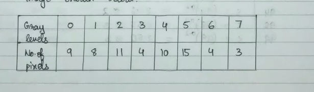
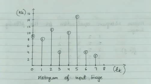
Method for 1-D

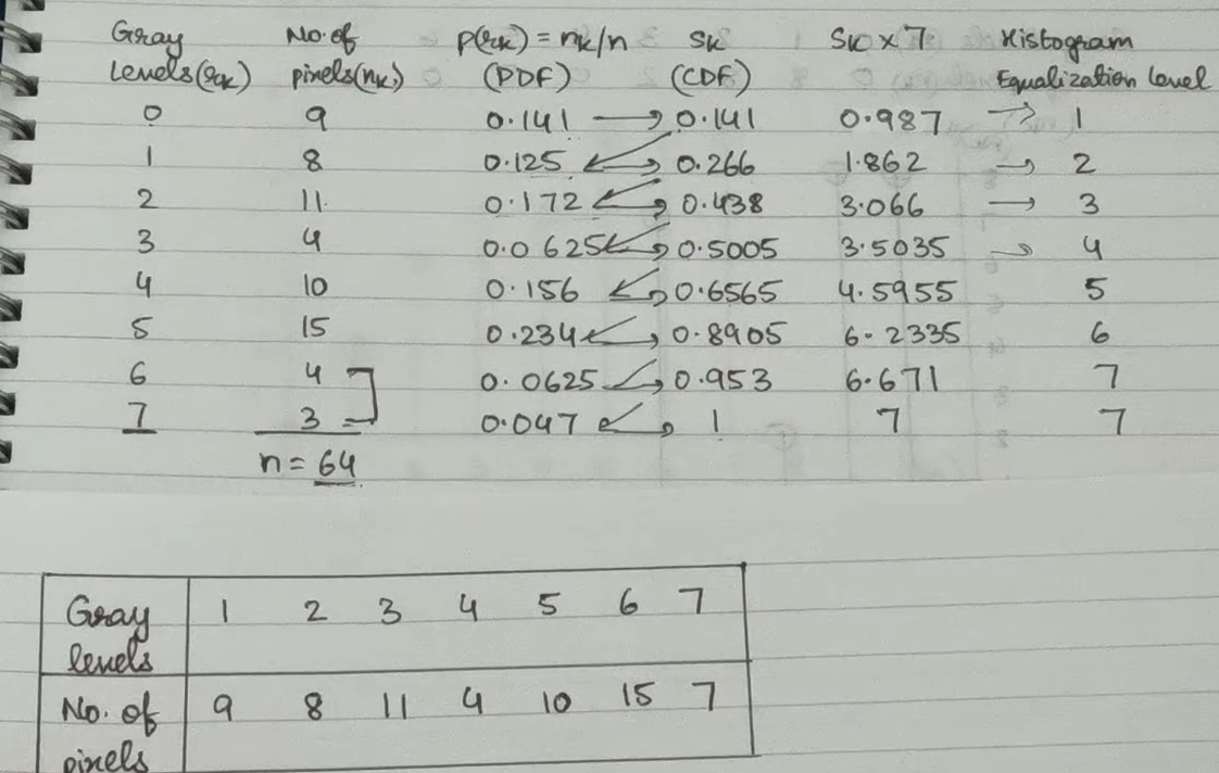
Find the values of PDF and CDF as follows
Multiply CDF with L-1 or maximum value in range.
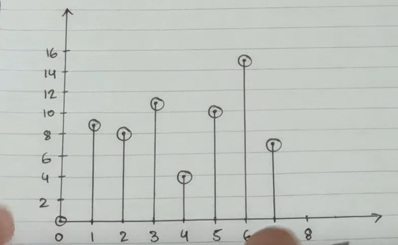
Round off the value thus obtained and this is the new gray level
If pixel gray values results are similar combine their frequency values to form new frequency.

Method for 2-D

Find the max value from the given matrix image and find the value of L corresponding to it which is a power of 2
then the values will lie in range from 0⇐r⇐L-1
now tabulate the frequency of this range values from the matrix given
Procede as with the 1-D method

Histogram Specification

In this we specify one equalised histogram in terms of another equalised histogram Method

Input: Equalise the modified from histogram and separate the gray levels and equalised values
Process: Equalise the to be modified histogram and separate the equalised values and new frequency values in separate table.
Map the values from the input histogram to the process histogram and place them in new table with gray values from range 0⇐ r ⇐ L-1
Draw new histogram.

Spatial Filtering

Convolution
- Rotate the kernel by 180 degrees
  - For 1-D rotate it vertically
  - For 2-D first rotate it vertically and then horizontally.
- Place above the image and then do the zero padding on each side.
  - For 1-D do zero padding on right and left sides.
  - For 2-D do zero padding by keeping the kernel over the image in such a way if original image is of M x N then the new image (zero padded) would be (M+(kernel_size - 1),N+kernel_size - 1) thus the number of rows and columns added are kernel_size-1
- Now at the zero padded image apply the mask/filter/kernel by multiplying the values.
  - For 1-D , move the filter across image and multiply the value and write the output under the center pixel of image of the current position of the kernel.
- For 2-D , move the filter across image and multiply the values and write the output on the new image’s position where kernel’s first position was originally.
  - Now move the kernel by one position and repeat the process until whole image is filtered.
    - In 1-D , the old image is only used for filtering
    - In 2-D , new images formed sub-subsequently are used for each next iteration.
Co-relation
- Don’t rotate the kernel by 180 degree
- rest steps same as convolution.

Smoothing filters

used to blur and noise reduce images
adds/integrates the similar neighbouring pixels
in filtering the centre pixel is the pixel that is changed.
Blurring is the pre-processing done to focus on the object by blurring out the minimal details.
Noise reduction can be done by both linear and non-linear filter along with blurring.
Types of Smoothing filters
- Linear (averaging filters): As they filter on basis of average of values in the neighbour.
  - Mean/Box
  - Kernel used
    $1 & 1 & 1 \\ 1 & 1 & 1 \\ 1 & 1 & 1 \\ \end{bmatrix}$
  - Weighted Average: The greater values are near the center diverging and decreasing outwards.
  - Kernel Used Example:
    $1 & 2 & 1 \\ 2 & 4 & 2 \\ 1 & 2 & 1 \\ \end{bmatrix}$
  - Gaussian: In this a Gaussian function is used to create filters
  - Kernel Used Example:
    $1 & 2 & 1 \\ 2 & 4 & 2 \\ 1 & 2 & 1 \\ \end{bmatrix}$
- Non-Linear : The response to these filters are produced by ranking of the pixels and then replacing the center pixel with value determined by ranking.
  - Median
  - Max
  - Min
Example
Smoothing Spatial Filters in digital image processing - YouTube

Sharpening Filters

Used for showing transitions in intensity levels
performs reverse operations to smoothing filters
subtracts/differentiate the surrounding neighbouring pixels
strength of this filters is according to the intensity discontinuity
focuses on sharp areas (high varying intensity) and not on blur areas (low varying intensity)
Types of Filters
1. Derivatives in 1-D
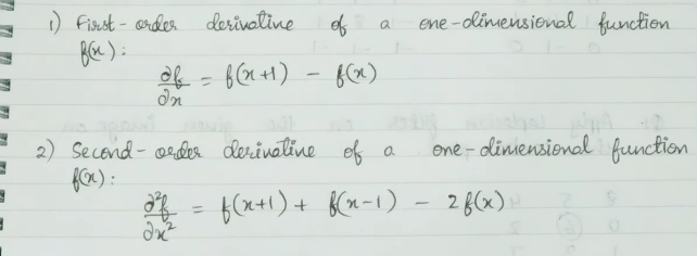
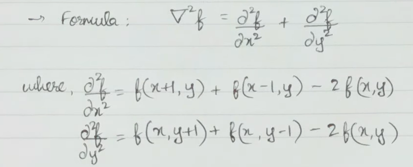
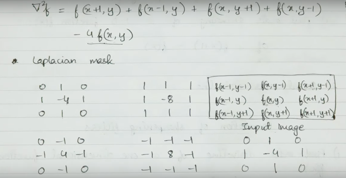
2. Second Order Derivative in 2-D(Laplacian)
Example Sharpening Spatial filters in digital image processing with examples - YouTube

Frequency Domain Transformations/Enhancements

In Frequency domain Transformations the image enhancements is done by first pre-processing and then transforming the image into frequency domain by use of Discrete Fourier Transform or Discrete Cosine Transform

Whole process is as follows :

Original image (G(x,y))
Pre-processing by moving the origin to center position by multiplying by (-1)^(x+y) to each pixel i.e by pixel by pixel multiplication
Transform into frequency domain (DCT or DFT) →F(x,y)
Convolution with H(x,y) by pixel by pixel multiplication
1. H(x,y) is calculated by calculating the Euclidean Distance of the original filter h(x,y) points from the relocated center.
Now inverse DCT or DFT accordingly the obtained image.
Get real part & return origin to its original position by multiplying it with (-1)^(x+y) by pixel by pixel multiplication

Type of Frequency domain filtering

Smoothing filters
1. Low pass filters
  1. Ideal Low pass
  2. Butter worth Low Pass
  3. Gaussian Low Pass
2. Smoothing or blurring the image by allowing low frequency components to pass.
3. Remove noise (high frequency components)
Sharpening filters
1. High pass filters
  1. Ideal high pass
  2. Butter worth Low pass
  3. Gaussian Low Pass
2. Sharpening of the image by allowing high frequency components to pass.
3. Removes Background of image.(object is of higher frequency than the background) Example: Frequency domain filtering in image processing - Low pass and High pass filters - YouTube

‧͙⁺˚･༓☾🐺☽༓･˚⁺‧͙

Explorer

Image Enhancement

Gray Level Or Spatial Domain Transformations/Enhancements

Point Operations